[Local LLM] How to tell if a hyped LLM optimization is real on your hardware: read the source, find the ceiling, run one experiment

The short version

Every week the local-LLM feed hands you a new optimization to be excited about: an external sparse-KV compressor, a memory trick, a "90% less KV at 500K context" headline. Some are real. Most are real for the author's model, which is not the same as real for yours. The failure mode isn't that people lie — it's that a number measured on an un-quantized reference model on a datacenter GPU quietly becomes a claim about your Q2 build on a 128GB box, and nobody re-checks.

You don't have to burn a week finding out which ones survive. Three cheap moves do most of the work, and I'll anchor each in one investigation — the FlashMemory one from Part 7, where I nearly bolted an external KV compressor onto a model that had already solved the exact problem it was solving.

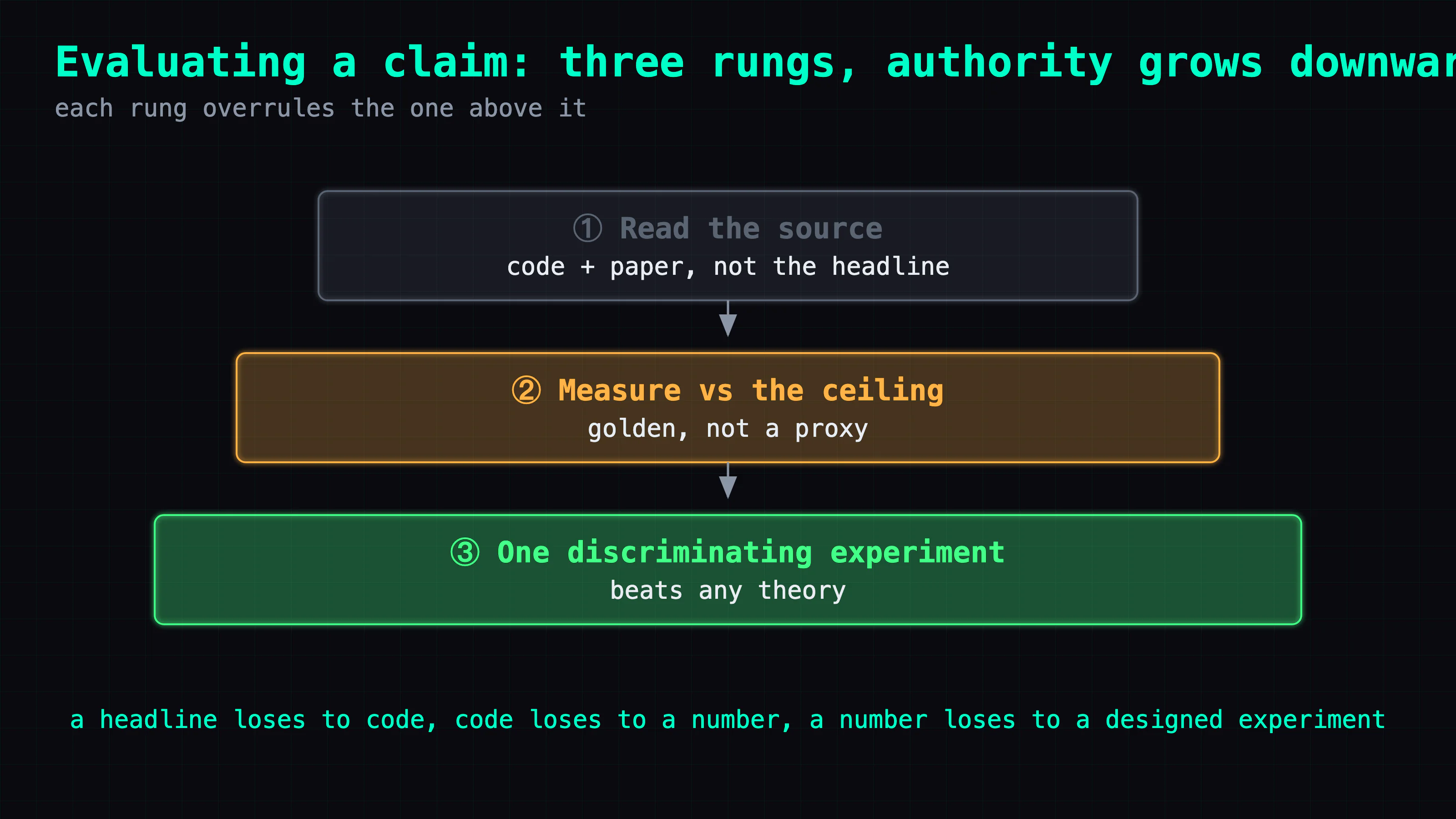
The three moves: read the actual code and paper before you touch anything; measure against the true ceiling instead of a convenient stand-in; and when theory gets slippery, design one experiment that can only come out one way if you're right. That's the whole discipline. The rest of this post is what each one looked like in practice.

---

The setup

Evaluating an optimization claim is like a contractor being pitched a miracle insulation. You don't argue with the brochure and you don't rip out the wall on faith — you read the spec sheet, you measure it against the best insulation already in the wall, and you cut one test panel. Skip any of the three and you either buy the hype or reject something good.

This is Part 8, and the last one in the DeepSeek-V4-Flash on DGX Spark series — the "so what" of everything before it. Part 6 took the architecture apart; Part 7 is the case study behind this post — the full play-by-play of the FlashMemory investigation I'm about to generalize. If you want the numbers with all their commentary, read Part 7. Here I'm pulling out the method, because the method is what carried across every other optimization I looked at for this model.

One honest caveat first: this isn't a universal law, it's what's worked for me on a single-box local setup where experiments are cheap and I own the whole stack. Your mileage may vary if you can't dump internal activations or retrain a projection on your own box. But the ordering — source, then ceiling, then experiment — holds regardless of scale.

---

Move 1 — Read the source and the paper first; it changes the question

The headline was "90% KV savings at 500K context." The temptation is to jump straight to "does it work on my box?" That question is premature, and reading two primary sources reframed it entirely.

First, the code — ds4's own. FlashMemory is an external sparse-KV compressor: it predicts which KV chunks matter and drops the rest. But reading ds4's implementation showed V4-Flash already has a native lightning indexer doing top-512 sparse selection at every step (this is the Part 6 material). That single fact flips the question. FlashMemory isn't adding sparsity to a dense model — it's proposing to replace selection the model already does. The bar isn't "beat dense attention," it's "beat native." Much higher, and I knew it before running anything.

Second, the paper — FlashMemory's own. The headline number was real but narrow. The paper's result tables report memory footprint and accuracy only: no serving-speed numbers in the paper. Its own dense-recall benchmark collapses (MRCR 48% vs 76%). And the project is an orphan — lead gone, suspended. None of that shows up in a "90% savings" post; all of it is one read of the actual arXiv PDF away.

So before a single GPU-second, the question had gone from "should I add this free memory win?" to "can an external, orphaned retriever whose paper only proves memory footprint and recall beat a jointly-trained selector the model already runs?" That's a different, far more skeptical question — and reading got me there for free. The headline tells you what a thing claims. The code and the paper tell you what it actually does, and just as important, what it doesn't.

Move 2 — measure against the true ceiling, not a convenient proxy

Once you run something, "it works / it doesn't" is meaningless without knowing what good is. This is where the FlashMemory investigation almost went wrong.

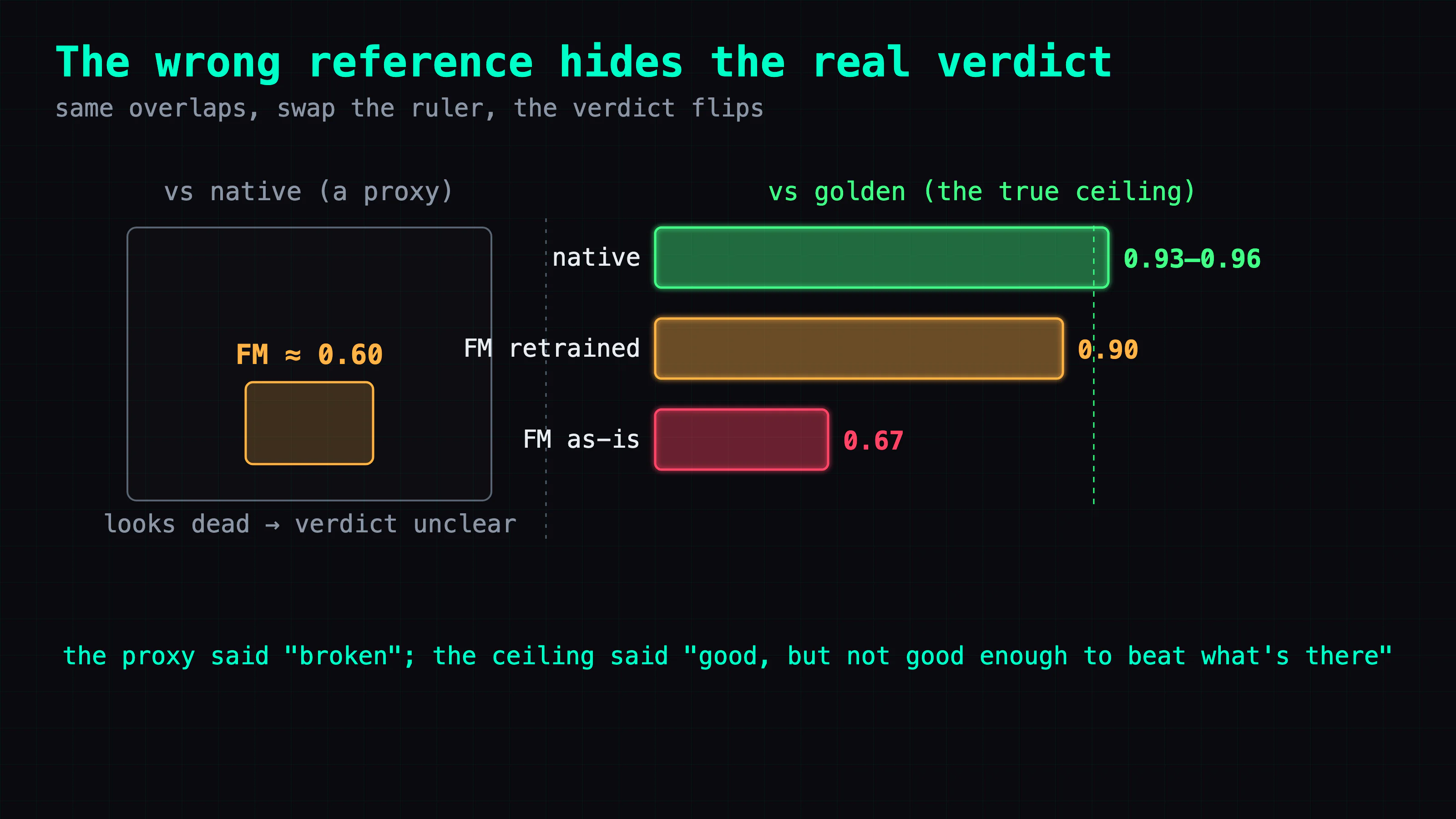
The obvious comparison: does FlashMemory pick the same chunks the native indexer picks? As-is, its overlap with native was 56.6% / 58.4% / 66.4% across three layers, against a 57.6% random baseline — basically random. Looks dead. But native is a proxy. Comparing FM to native only tells you whether FM imitates native, not whether either is any good. If native itself were mediocre, "FM disagrees with native" would be no verdict at all.

The true ceiling is dense attention — what the model would attend to if it computed unmasked softmax over every chunk, no sparsity. That's the ground truth both selectors approximate. So I dumped real dense attention as golden and scored each method against it. Native tracks golden at 0.93–0.96 — near-optimal. Even the best version of FM I could produce landed at 0.90. Against the proxy, FM looked simply broken; against the ceiling, the picture changed: native is nearly perfect, so there's only a 4–7 point gap for any external scheme to fit into, and it has to be flawless to fill it.

The lesson isn't subtle once you see it, but it's easy to miss in the moment: pick the reference that answers the actual question. The question was never "does FM match native," it was "is FM better than what I already run." Only a comparison against the true ceiling answers that, and the ceiling was cheap to dump.

Move 3 — one discriminating experiment beats any amount of theory

Between reading and the final verdict there was a tempting theoretical detour. As-is, FM picked near-randomly on my Q2 build. Why? Two stories fit the same data. Maybe the architecture can't learn my quantization — a real, fatal limit. Or maybe it was just trained on the wrong distribution (un-quantized V4) and my Q2 keys shifted under it — annoying but fixable. You can argue those two forever from the armchair; the as-is number is equally consistent with both.

So don't argue — build the one measurement that comes out differently depending on which story is true. If it's distribution shift, showing FM my distribution should fix it; if it's an architectural limit, it won't. I fine-tuned only FM's small projection weights on ~160 samples of my Q2. Val overlap jumped from ~0.67 to 0.91–0.94. That settles it empirically: it was a pure distribution shift — annoying but fixable, not an inherent architectural limitation. No amount of theorizing about "the architecture" would have gotten there; ~160 samples did, in an afternoon.

And the golden comparison was the final referee for the whole thing. There's always a last theoretical escape hatch — "retrained FM should generalize," "it'd win on a lookahead target." Maybe. But retrained FM, trained directly toward the golden target, still scored 0.886 / 0.910 / 0.916 — under native's 0.930 / 0.957 / 0.956 on all three layers. No story about what should happen survives the number 0.90 < 0.93–0.96. Design the experiment whose result can't be argued with, and let it be the judge.

The verdict for FlashMemory on this stack was NO-GO — not because the technique is bad, but because V4-Flash already ships a near-optimal native selector, so there's nothing for an external one to win. But that verdict is Part 7's story. This post is about how the three moves got me there without a wasted week — and they're the same three I run on every optimization claim in this series.

Takeaways

Where the time went

Not in reading and not in the retrain — the retrain is ~160 samples and finishes in an afternoon. The time (and the near-miss) was in Move 2. After the retrain hit 94% agreement with native, I had a result that looked positive and I nearly wrote it up that way. The hour I'd have "saved" by stopping there was the hour I spent dumping the golden to check whether "agrees with native" and "beats native" were the same question. They weren't, and the gap between them was the entire finding. Choosing the wrong reference doesn't cost you a wrong number — it costs you the wrong conclusion, which is worse.

Reusable diagnostics

Three, in the order you run them. Before anything: read the target's own code for whether the problem is already solved internally — a native mechanism turns "add X" into "beat X" and raises every downstream bar. Before you trust any "it works" result: dump the true ceiling and score against that, not against the incumbent — the incumbent is a proxy and can flatter or damn unfairly. When theory forks: design the cheap probe whose result differs by branch — the retraining run (0.67 → 0.92) separated "can't learn" from "wrong distribution" in a single run — something no amount of theorizing could do.

The general principle

Read the source, find the true ceiling, run one discriminating experiment — in that order, because each stage narrows what the next one has to test. Reading reframes the question so you measure the right thing; the ceiling tells you what winning even means; the one experiment settles what's left when theory forks. This is why most hyped "N× faster / 90% less memory" claims don't change what I actually run: they're usually real for some model, and the three moves tell me, cheaply, whether that model is mine.

Conclusion: the checklist

1. Read the primary source before you run anything. The actual code and the actual paper, not the headline. Reading ds4's code turned "add sparsity" into "beat the native indexer"; reading FlashMemory's paper surfaced paper-scoped memory/accuracy results and a dense-recall collapse. The question you should be testing is usually not the one the headline poses.
2. Find the true ceiling and measure against it. Not the incumbent method — the ground truth. Native-vs-golden was 0.93–0.96, and that one number is what made the verdict unambiguous. The proxy comparison (FM-vs-native ~0.60) told a different, wrong story.
3. When theory forks, run the one experiment that separates the branches. "Can't learn" vs "wrong distribution" looked identical in the as-is data; a ~160-sample retrain (0.67 → 0.92) told them apart empirically. Design the measurement that can only come out one way if you're right.
4. Don't confuse "matches the incumbent" with "beats the ceiling." Retrained FM hit 94% agreement with native and still lost to native against golden. Agreement is not improvement.
5. Most hyped claims are real but narrow. "90% KV savings" was true — for a model without a native indexer. The three moves are how you find out, cheaply, whether the narrow case is yours.

---

Also in this series: Part 5 — Depth-1 MTP: route speculative decode by workload · Part 6 — Inside V4-Flash's architecture and its lightning indexer · Part 7 — FlashMemory can't beat V4-Flash's own lightning indexer · Upstream: antirez/ds4